Paste your numbers to see a histogram with the mean line, three standard deviation bands and an optional normal curve.
Loading calculator…
Type or paste your data, and this standard deviation graph shows how the values spread around the mean. You get a histogram, a dashed line at the average, three shaded bands (1, 2 and 3 standard deviations from the mean), and an optional normal curve to compare against. In other words, it works as a standard deviation histogram calculator: the bars are the histogram, and the bands show the standard deviation. To see the arithmetic behind the number, use the standard deviation tool; for the average alone, see the mean tool. More tools are in descriptive statistics calculators.
What each part of the picture means
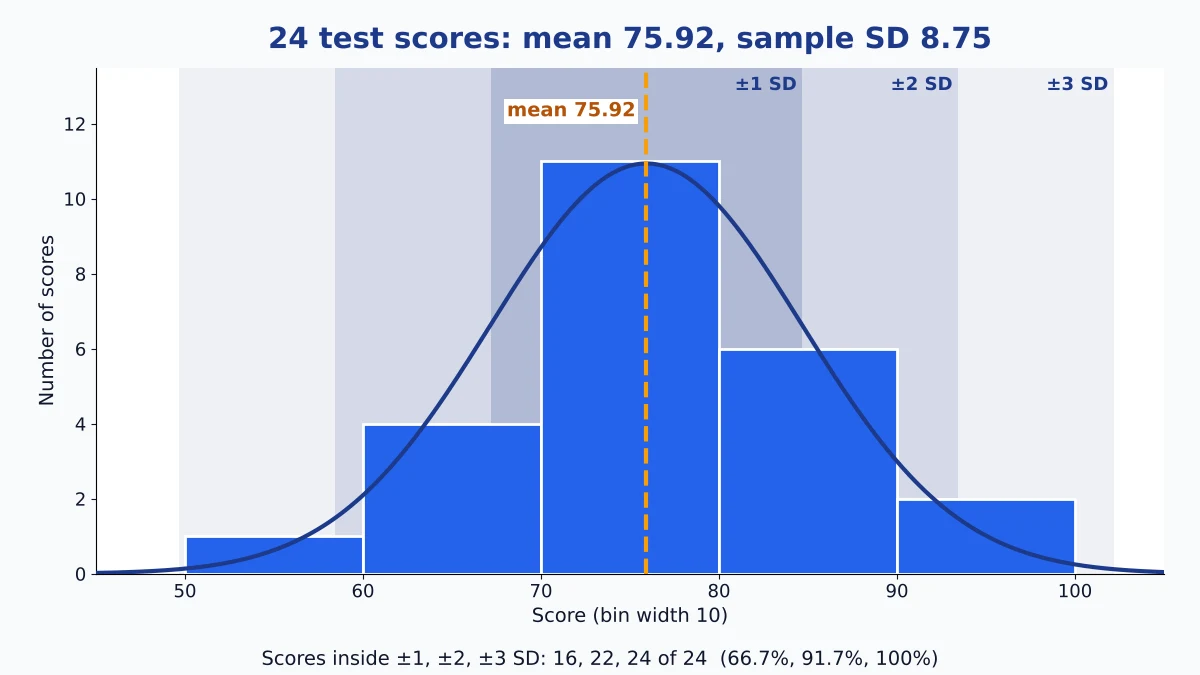
The bars are your data, grouped into bins. A bar’s height is simply how many values fall inside that bin. The dashed line marks the mean. The innermost band extends one standard deviation to the left and right; the lighter bands extend two and three.
The built-in test-score example has 24 scores. The mean is 75.92 with a sample standard deviation of 8.75, so the first band covers 67.16 to 84.67. Most of the tall bars sit inside it. Seeing that is the point of a standard deviation chart: two summary numbers become a shape you can judge.
The tool chooses the number of bins for you from the number of values (Sturges’ rule: log base 2 of n, plus 1), then rounds the width to something readable such as 5, 10 or 20. If the shape looks too blocky or too jagged, type your own bin count between 3 and 30.
Count the bands against the normal pattern
Under the graph, a table counts how many values fall within each band. For the 24 test scores it shows 16, 22 and 24 values, or 66.7%, 91.7% and 100%. On a normal distribution graph, about 68.27%, 95.45% and 99.73% of values fall in those bands, which would be 16.4, 22.9 and 23.9 of 24.
So this data behaves almost exactly as the rule predicts. Do not expect that every time. With so few values, one score moving across a band edge changes a percentage by about 4 points. The standard deviation tool page explains where the 68-95-99.7 figures come from.

| Slice of a normal curve | Share of values |
|---|---|
| Mean to 1 standard deviation (either side) | 34.13% |
| 1 to 2 standard deviations (either side) | 13.59% |
| 2 to 3 standard deviations (either side) | 2.14% |
| Beyond 3 standard deviations (both tails) | 0.27% |
Same mean, different story
Load the three examples one after another. The test scores bunch around 76 and thin out toward both ends. The incomes example (12 values, in thousands) has a mean of 42.25, but eight of the twelve values sit below 40, while a single 95 drags the mean upward. The two-peaks example has a mean of 10.25 and almost nothing near it.
That last one is the clearest lesson. Its standard deviation is 6.79, and the first band holds 11 of 16 values, yet the bin around the mean is empty. The numbers look reasonable and the picture shows two separate groups. Always look at the bars before you trust the summary.
What changing the bins does
Bins are a drawing choice, not part of your data. With very few bins, a two-humped dataset can look like one smooth hill. With too many, every value gets its own thin bar and the shape turns jagged. The mean, the standard deviation and the band counts do not change when you change the bins; only the bars do.
A practical routine: leave the setting on Auto, then try one count a few steps lower and one higher. If the overall shape survives all three, you can trust it.
How to find standard deviation from a graph
When all you have is a picture of a bell curve and you need the standard deviation from a graph, look on each side for the spot where the curve stops dropping faster and begins to level off. Measure sideways along the horizontal axis from the peak to that point; that distance is one standard deviation. On a histogram, one standard deviation is the distance from the mean line to the edge of the innermost band.
For a histogram, a quick check is the range divided by about 4 when you have a few dozen values. In the test-score example the range is 94 − 58 = 36, which gives 9 against a true 8.75. Use it to catch a typing mistake, not to replace the calculation. One extreme value stretches the range and spoils the estimate.
How to graph standard deviation in Excel
- Put the values in one column. Use
=AVERAGE(A2:A25)for the mean and=STDEV.S(A2:A25)for the sample standard deviation (=STDEV.Pfor a whole population). - Select the column and choose Insert, then Statistic chart, then Histogram (Excel 2016 or later). Set the bin width under Format Axis.
- For a curve, list the bin centers in a column and enter
=NORM.DIST(x, mean, sd, FALSE)*n*bin widthbeside them. Add that column to the chart as a line.
The tool above does all three steps at once, and Download PNG saves the finished picture.
Excel also has an Error Bars option under Chart Elements. It adds a bar for the standard deviation to a column or line chart, which makes a standard deviation bar graph of group means, not a picture of how one list is spread. Use the histogram steps for the spread of a single list. For the standard deviation on a graphing calculator, see the TI-83/84 steps on the standard deviation calculator page.
When the bell curve is the wrong yardstick
The overlay uses only your mean and standard deviation, even when those two numbers describe your data poorly. In the incomes example the curve centers on a value few people actually earn, and its lower band reaches toward zero. When you see a long tail, a gap or two humps, report the median and the interquartile range instead, or try the mean absolute deviation calculator, which reacts less to one extreme value.
Do not read overlapping standard deviation bars on a chart of two groups as proof that the groups do not differ. Spread and certainty about the mean are different things.
Standard deviation graph FAQs
How do I graph standard deviation for my own numbers?
Paste them into the box, choose sample or population, and press Calculate. The tool draws the bars, the mean line and the three bands. Tick Show normal curve to add the curve, then Download PNG to save it.
How do I read the standard deviation off someone else’s graph?
Measure sideways from the peak of the bell curve to the spot where it begins to level off. That gap is one standard deviation. On a histogram, use about a quarter of the range for a few dozen values.
Is a standard deviation graph the same as a bell curve?
No. A bell curve is a smooth ideal shape. This graph shows your actual values as bars and can place a bell curve over them so you can see how far your data departs from it.
Why do my bars not follow the curve?
Small samples, skew, outliers and two groups all cause gaps. Mismatch is information: it tells you the normal model is a poor description of your data.
Should I choose sample or population?
Choose sample when your values are a subset of a larger group, and population when you have every value. The sample result is slightly larger, so the bands are a little wider.
What happens when the standard deviation gets larger?
The curve spreads out and gets lower, and the bands move farther from the mean. The center stays where the mean is.
How many bins should I use?
Start with Auto, then try a few counts between 5 and 12. Keep the one where the shape stays the same across settings.
Easy Stat Calc · Results checked against Python, R and Excel · Last updated November 2, 2026 · Methodology