
Enter the possible outcomes of a random variable and their probabilities to get the expected value, variance and standard deviation, with the working and a chart.
Loading calculator…
This probability distribution calculator works on any table you type: outcomes in one column, probabilities in the other. It doubles as an expected value calculator and an expected value and standard deviation calculator in one, so you also get the variance of the probability distribution in the same run. You can type decimals, fractions such as 1/6 or percents, add as many rows as you need, or enter counts and let the tool turn them into probabilities.
Beyond the three headline numbers, it adds up the chance of landing at or below a value, at or above it or between two values, shows each multiplication in a working table, and draws a bar chart with the expected value and a one-standard-deviation band marked.
How to use this probability distribution calculator
- Type each possible outcome x in the left column and its probability P(x) in the right column. Add a row for each extra outcome. Outcomes can be negative or decimal.
- Check the type of probability. Leave it on “I have probabilities”, or switch to counts if you have frequencies, such as how many students gave each answer.
- Press Calculate. The expected value E(X), the variance and σ appear first, then the working table, the four steps and the chart.
- Ask a question if you need one. Open “Also find a probability” to get P(X = a), P(X ≤ a), P(X ≥ a) or P(a ≤ X ≤ b) from your own table.
- Use an example button to see how it works: a fair die, a loaded die, a game with a loss, or survey counts.
If the probabilities do not add up to 1, no results appear. The message says how far off you are, and a button offers to add the missing probability as a new outcome row. A column pasted from a spreadsheet also works: open “Paste two columns” and drop it in.
What is a probability distribution?
A discrete probability distribution lists every value a discrete random variable can take and the chance of each one. This table is what the tool needs, so it works as a discrete probability distribution calculator and as a discrete random variable calculator for the center and spread of your table. The variable X might be the number a die shows, the number of siblings a student has, or the payoff of a game. For a discrete variable the table is called a probability mass function (PMF): it gives P(X = x) for each listed value. A continuous variable, such as a temperature, has infinitely many values, so it uses a density curve (a PDF) instead and its probability at one exact value is effectively zero. This calculator handles the discrete case. Written out in rows, it is a probability distribution table. Two rules make a table valid: every probability is between 0 and 1, and all the probabilities add up to exactly 1.
| Outcome x | 1 | 2 | 3 | 4 | 5 | 6 |
|---|---|---|---|---|---|---|
| P(x) | 1/6 | 1/6 | 1/6 | 1/6 | 1/6 | 1/6 |
The table above is the distribution of one roll of a fair die. Once you have the table, a few numbers summarize it: the expected value (the center), the variance and SD (the spread), and cumulative probabilities (the chance of reaching a threshold). That is what this calculator computes. Distributions with a fixed recipe, such as the Poisson distribution or the hypergeometric distribution, have their own calculators that build the table from a few inputs.
Expected value formula: how to find expected value and calculate it
E(X) = Σ x · P(x). This expected value formula, also called the expected value equation, is the formula for expected value in every probability distribution table. To calculate expected value by hand, multiply each outcome by its probability, then add the products. The result is the mean of the probability distribution, often written μ, so this is also how to find the expected value of a probability distribution. Take the fair die: E(X) = (1 + 2 + 3 + 4 + 5 + 6) ÷ 6 = 21 ÷ 6 = 3.5.
For the squares, E(X²) = Σ x² · P(x). For the die, 1 + 4 + 9 + 16 + 25 + 36 = 91, and 91 ÷ 6 = 15.1667. Those two sums are everything the spread measures below need.
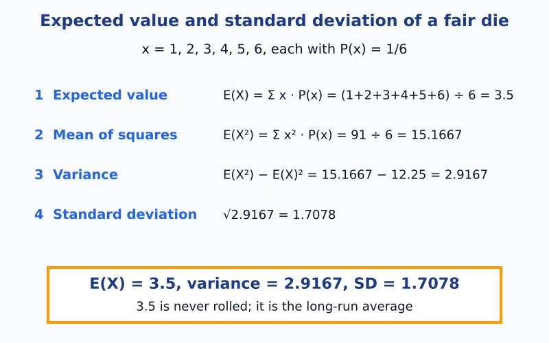
Paste 1 to 6 with 1/6 each into the expected value calculator, or press the fair die example, and the working table shows each x · P(x) and x² · P(x) with their totals, so you can check each line of the hand calculation.
Variance and standard deviation of a probability distribution
The variance measures how far the outcomes typically fall from the expected value, weighting each one by its probability. There are two equal ways to write it:
- Deviation form: Var(X) = Σ (x − E(X))² · P(x).
- Shortcut form: Var(X) = E(X²) − E(X)², which needs no deviations.
For the die the shortcut gives 15.1667 − 3.5² = 15.1667 − 12.25 = 2.9167, and the deviation form gives the same value: (6.25 + 2.25 + 0.25 + 0.25 + 2.25 + 6.25) ÷ 6 = 2.9167. Taking the square root gives σ = √Var(X) = 1.7078. Because the probabilities describe the whole distribution, there is no sample correction here: nothing is divided by n − 1. For the standard deviation of a list of numbers you measured, use the standard deviation tool instead.
Mean of a discrete probability distribution: a survey example
Homework often reads: “calculate the mean for the discrete probability distribution shown here”. The recipe is the expected value formula. Suppose 20 students were asked how many siblings they have: 2 said none, 5 said one, 9 said two and 4 said three. Divide each count by 20 to get the probabilities 0.1, 0.25, 0.45 and 0.2.
| Siblings x | Students | P(x) | x · P(x) |
|---|---|---|---|
| 0 | 2 | 0.1 | 0 |
| 1 | 5 | 0.25 | 0.25 |
| 2 | 9 | 0.45 | 0.9 |
| 3 | 4 | 0.2 | 0.6 |
| Total | 20 | 1 | 1.75 |
The mean of the distribution, which is also the mean of the discrete random variable X, is 1.75 siblings. The mean of the squares is 3.85, so the variance is 3.85 − 1.75² = 0.7875 and σ = 0.8874. Switch the tool to counts mode and enter 2, 5, 9, 4 to see the same table. If your data is a plain list of values with their frequencies, the mean, median and mode tool has a frequency-table mode, and for a single list of numbers use the mean tool.
Expected value of a game with a loss
Payoffs can be negative. A game pays −$5 with probability 0.5, $0 with probability 0.3, $10 with probability 0.15 and $50 with probability 0.05. Multiply and add: −2.5 + 0 + 1.5 + 2.5 = 1.5. The expected value is $1.50 per play, a small average gain.

The standard deviation of this game is 12.2577, much larger than the expected value, so single plays swing widely even though the long-run average is positive. That is why it pays to read the expected value and the standard deviation together. The chart marks E(X) with a dashed line and shades one standard deviation either side. In this game the bars at −$5, $0 and $10 fall inside the band and the $50 bar sits outside it.
Cumulative and range probabilities from your table
Use the “Also find a probability” row, and the working table of the probability distribution calculator, to read cumulative probabilities straight from your own distribution. P(X ≤ x) adds the probabilities up to and including x, and P(X ≥ x) adds from x upward. The running total P(X ≤ x) is the cumulative distribution function (CDF) of your table. For the fair die:
| Question | Outcomes added | Result |
|---|---|---|
| P(X ≤ 3) | 1, 2, 3 | 0.5 |
| P(X ≥ 5) | 5, 6 | 0.3333 |
| P(2 ≤ X ≤ 4) | 2, 3, 4 | 0.5 |
| P(X = 6) | 6 | 0.1667 |
For the game above, the chance of not losing money is P(X ≥ 0) = 0.3 + 0.15 + 0.05 = 0.5, and the chance of winning at least $10 is P(X ≥ 10) = 0.2. The tool writes out each sum next to the answer so a teacher can follow it.
Where expected value and spread are used
- Games of chance: the expected value is the average gain or loss per play, and the standard deviation shows how bumpy single plays are.
- Surveys: counts of answers become probabilities, and the expected value is the average answer.
- Planning: any decision with a few outcomes and estimated probabilities, such as the number of orders in a week, can be summarized as a mean and a spread.
The numbers describe the distribution you type, so they are only as good as your probabilities.
Is my table a valid probability distribution?
Before it calculates, the tool checks the two rules. A probability below 0 or above 1 is rejected with the row number. A total that is not 1 is rejected too, unless it is within 0.0001 of 1 from rounding, in which case the tool uses your numbers and tells you the total. For example, outcomes 1 and 2 with probabilities 0.5 and 0.35 add up to 0.85. The message says you are 0.15 short and offers a button to add a row for the missing 0.15.
If you type the same outcome twice, the tool combines the two rows and says so. A distribution with a single outcome is allowed: its variance and standard deviation are 0, because nothing varies.
Check expected value and SD with Excel or a TI-84
To check the result yourself, put the outcomes in A2:A7 and the probabilities in B2:B7 (headings in row 1). The calculator shows these formulas with your own ranges:
| Task | Excel / Google Sheets | TI-83/84 |
|---|---|---|
| Expected value | =SUMPRODUCT(A2:A7,B2:B7) | STAT, EDIT: x in L1, P(x) in L2; open 1-Var Stats with List L1 and FreqList L2; read x-bar |
| Variance | =SUMPRODUCT(A2:A7^2,B2:B7)-SUMPRODUCT(A2:A7,B2:B7)^2 | square the sigma-x value from the same screen |
| Standard deviation | =SQRT(SUMPRODUCT(A2:A7^2,B2:B7)-SUMPRODUCT(A2:A7,B2:B7)^2) | read sigma-x (not Sx) on the same screen |
On the TI-84, the 1-Var Stats screen shows both x-bar and σx for the weighted list. Use σx: the probabilities describe the whole distribution, so the sample version Sx does not apply.
When to use a different calculator
This probability distribution calculator is for tables you build yourself. When your situation follows a standard model, a dedicated calculator is quicker: use the Poisson calculator for event counts when events arrive at a known average rate, the hypergeometric tool when you sample from a small group without putting items back, or the basic probability calculator to combine the chances of single events. All of them sit in the probability calculators hub.
Probability distribution calculator FAQs
How do you find a probability distribution?
List every possible outcome, then find the probability of each. If you know the counts, such as how many students gave each answer, divide each count by the total. If the outcomes are equally likely, like the six faces of a die, give each one 1/6. Then check that the probabilities add up to 1. The result is your probability distribution table, and you can type it straight into the calculator.
What is the expected value of a probability distribution?
The expected value is the long-run average of a random variable. Multiply each outcome by its probability and add the results. For a fair die it is 3.5, a number you can never roll, which is fine: it is where the average of many rolls settles, not a result of any single roll.
How do you find expected value?
List every possible outcome x with its probability P(x), multiply each pair, and add: E(X) = Σ x · P(x). For the outcomes −5, 0, 10 and 50 with probabilities 0.5, 0.3, 0.15 and 0.05, the products are −2.5, 0, 1.5 and 2.5, and the sum is 1.5.
How do you calculate the standard deviation of a probability distribution?
First find the expected value E(X) and the mean of the squares E(X²) = Σ x² · P(x). The variance is E(X²) − E(X)², and the standard deviation is its square root. For a fair die that is 15.1667 − 12.25 = 2.9167, and the square root is 1.7078.
Is expected value the same as the mean?
For a probability distribution, yes: the expected value is the mean of the distribution, often written μ. For a list of observed numbers the average is called the sample mean, and our mean calculator handles that case. The expected value comes from probabilities you are given, not from data you collected.
Can the expected value be negative?
Yes. If the outcomes include losses and the losing outcomes are likely enough, the weighted average falls below zero. An expected value of exactly zero describes a fair game, where gains and losses balance on average.
What is a good expected value?
There is no universal answer, because it depends on what you compare it with. Compare E(X) with what it costs to take part, and check the standard deviation too: two games can share an expected value of 1.5 while their single results scatter very differently.
Do the probabilities have to add up to 1?
Yes. A discrete probability distribution covers every possible outcome, so the probabilities must total 1, and each one must be between 0 and 1. If yours do not, the calculator shows no results, tells you how far off the total is and offers to add the missing probability as a new outcome row.
Can I enter fractions or percents instead of decimals?
Yes. Type 1/6, 0.1667 or 16.67% and the tool understands all three. Fractions are kept exact behind the scenes, so six entries of 1/6 add up to exactly 1.
What if I only have counts, not probabilities?
Switch to “I have counts or frequencies”. The tool divides each count by the total to get the probabilities and shows them in the table. For 2, 5, 9 and 4 students with 0, 1, 2 and 3 siblings, the probabilities are 0.1, 0.25, 0.45 and 0.2, and the expected number of siblings is 1.75.
Is there an Excel formula for expected value?
Yes. With outcomes in A2:A7 and probabilities in B2:B7, =SUMPRODUCT(A2:A7,B2:B7) gives the expected value. For the standard deviation, take =SQRT(SUMPRODUCT(A2:A7^2,B2:B7)-SUMPRODUCT(A2:A7,B2:B7)^2).
What is the difference between discrete and continuous distributions, and which does this handle?
A discrete distribution has separate outcomes you can list, such as 0, 1, 2 or 3 siblings, and each outcome has its own probability. A continuous distribution covers every value in a range, such as heights or times, and probability is found as area under a curve instead of from a list. This calculator is for discrete distributions, where you can type the outcomes.
What is the difference between variance and standard deviation?
The variance is the probability-weighted average of the squared distances from the expected value, so it is in squared units. The standard deviation is its square root, which brings the spread back into the units of the outcomes. For the game above, a variance of 150.25 dollars squared becomes a standard deviation of 12.2577 dollars.
Why does the TI-84 show sigma-x and Sx?
With 1-Var Stats on L1 and FreqList L2, the x-bar is the expected value and σx is the standard deviation of the distribution, which is what you want. Sx is the sample standard deviation formula for raw data and is not the answer for a probability table.
Easy Stat Calc · Results checked against Python, R and Excel · Last updated November 3, 2026 · Methodology